Every serious computer science curriculum, every technical interview at a product company, and every competitive programming contest rests on the same foundation: the Design and Analysis of Algorithms. Whether you are a first-year engineering student encountering this subject for the first time, a self-taught developer trying to fill a gap before interviews, or someone preparing for GATE, this DAA Tutorial 2026 walks through every core concept from first principles — how to measure an algorithm's efficiency, how to design algorithms systematically rather than by guesswork, and how to apply these techniques to real problems. This is the complete DAA for Beginners resource, with worked code examples, complexity analysis, and a clear DAA Roadmap for what to learn and in what order.
What We Cover
- Why Design and Analysis of Algorithms Matters
- Time Complexity Tutorial — Measuring Algorithm Speed
- Space Complexity — Measuring Memory Usage
- Data Structures and Algorithms — The Essential Pairing
- Algorithm Design Techniques — Divide and Conquer, Greedy, DP
- Greedy Algorithms — Making the Locally Best Choice
- Dynamic Programming Tutorial — Solving Overlapping Subproblems
- DAA Roadmap — Your 12-Week Learning Path
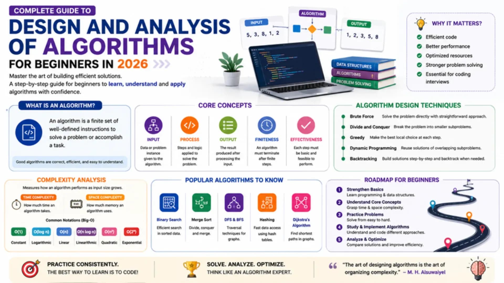
Why Design and Analysis of Algorithms Matters
Every program you will ever write solves a problem through some sequence of steps — that sequence is an algorithm. The Design and Analysis of Algorithms as a discipline answers two distinct questions: how do you systematically construct an algorithm that solves a problem correctly (design), and how do you predict how that algorithm will perform as the input grows larger (analysis)?
This matters in practice far more than it might seem from a textbook. Two algorithms that both produce correct output for a 100-item list can behave completely differently for a 10-million-item list — one finishing in milliseconds, the other taking hours. Without the Design and Analysis of Algorithms framework, you have no systematic way to predict this difference before it happens in production, which is precisely how slow, expensive systems get built by capable programmers who never learned to reason about complexity.
DAA for Beginners students often ask whether this subject matters if modern computers are fast and memory is cheap. The honest answer: at small scale, often not noticeably — but at the scale of real production systems (search engines, social media feeds, recommendation systems, financial transaction processing), the difference between an O(n²) algorithm and an O(n log n) algorithm is the difference between a system that works and one that does not.
Time Complexity Tutorial — Measuring Algorithm Speed
The core tool of any Time Complexity Tutorial is Big-O notation — a way of describing how an algorithm's running time grows as the input size (n) grows, without depending on the specific hardware running it. Big-O describes the worst-case growth rate, ignoring constant factors and lower-order terms, because what matters for large inputs is the dominant term.
Common Complexity Classes, From Fastest to Slowest
| Notation | Name | Example |
|---|---|---|
| O(1) | Constant | Array index access |
| O(log n) | Logarithmic | Binary search |
| O(n) | Linear | Single loop through array |
| O(n log n) | Linearithmic | Merge sort, quicksort (average) |
| O(n²) | Quadratic | Nested loops, bubble sort |
| O(2ⁿ) | Exponential | Naive recursive Fibonacci, brute-force subsets |
Calculating Time Complexity — A Worked Example
Consider this function that checks whether an array contains any duplicate values:
def has_duplicates_naive(arr):
    n = len(arr)
    for i in range(n):           # runs n times
        for j in range(i + 1, n): # runs up to n times for each i
            if arr[i] == arr[j]:
                return True
    return False

# Time Complexity: O(n^2) - nested loops over the same array
# Space Complexity: O(1) - no extra data structure used
A more efficient version using a hash set, central to any good Time Complexity Tutorial:
def has_duplicates_optimized(arr):
    seen = set()
    for num in arr:               # single pass, runs n times
        if num in seen:            # O(1) average lookup in a hash set
            return True
        seen.add(num)              # O(1) average insertion
    return False

# Time Complexity: O(n) - single pass through the array
# Space Complexity: O(n) - the 'seen' set can grow up to size n
This comparison is the heart of why Design and Analysis of Algorithms matters practically: the optimized version trades a small amount of extra memory (O(n) space) for a dramatic improvement in speed (O(n) time instead of O(n²)) — for an array of 100,000 elements, this is the difference between roughly 10 billion operations and 100,000 operations. Any thorough Algorithm Analysis Guide will emphasise this exact trade-off as the foundational lesson before moving to more advanced design techniques.
Space Complexity — Measuring Memory Usage
Space Complexity measures how much additional memory an algorithm needs relative to its input size, using the same Big-O notation as time complexity. This is frequently underemphasised relative to time complexity, but it matters enormously in memory-constrained environments — embedded systems, mobile applications, and large-scale distributed systems where memory cost multiplies across thousands of machines.
A critical distinction in Space Complexity analysis: input space (the memory the input itself occupies) is usually excluded from the calculation; what matters is the auxiliary space — any additional memory the algorithm allocates beyond the input. Recursive algorithms deserve particular attention here, since each recursive call adds a frame to the call stack:
def factorial_recursive(n):
    if n <= 1:
        return 1
    return n * factorial_recursive(n - 1)

# Time Complexity: O(n) - n recursive calls
# Space Complexity: O(n) - the call stack holds n frames simultaneously
#                    (not O(1), even though no explicit data structure is created)

def factorial_iterative(n):
    result = 1
    for i in range(2, n + 1):
        result *= i
    return result

# Time Complexity: O(n)
# Space Complexity: O(1) - no growing call stack; just one accumulator variable
This recursive-versus-iterative trade-off recurs constantly in algorithm design: recursive solutions are often more readable and closer to a mathematical definition, but they carry a Space Complexity cost from the call stack that iterative versions avoid. For deeply recursive problems (processing very large datasets recursively, for example), this can cause actual stack overflow errors in production — not just a theoretical inefficiency.
Related Article: Top MTech Colleges in India
Data Structures and Algorithms — The Essential Pairing
Data Structures and Algorithms are taught together, and for good reason: the choice of data structure often determines what algorithmic complexity is even achievable. Choosing the wrong data structure can make an otherwise well-designed algorithm slow, regardless of how cleverly the logic is written.
A concrete illustration — searching for an element, implemented across different data structures:
# Searching in an unsorted array/list
def search_list(lst, target):
    for item in lst:
        if item == target:
            return True
    return False
# Time Complexity: O(n) - must check every element in the worst case

# Searching in a sorted array using binary search
def search_sorted_array(arr, target):
    low, high = 0, len(arr) - 1
    while low <= high:
        mid = (low + high) // 2
        if arr[mid] == target:
            return True
        elif arr[mid] < target:
            low = mid + 1
        else:
            high = mid - 1
    return False
# Time Complexity: O(log n) - halves the search space each iteration

# Searching using a hash set
def search_hash_set(hash_set, target):
    return target in hash_set
# Time Complexity: O(1) average case - direct hash lookup
The same logical task — "is this value present?" — has three completely different complexity profiles purely based on data structure choice. This is why Data Structures and Algorithms are inseparable in practice: arrays, linked lists, stacks, queues, trees, heaps, and hash tables each make certain operations fast and others slow, and effective algorithm design starts with choosing the data structure whose strengths match the problem's actual requirements.
Algorithm Design Techniques — Divide and Conquer, Greedy, DP
Rather than inventing a new approach for every problem, experienced algorithm designers recognise that most problems fit one of a handful of established Algorithm Design Techniques. Learning to recognise which technique fits a given problem is the single highest-leverage skill in this entire subject.
Divide and Conquer
Break a problem into smaller independent subproblems, solve each recursively, then combine the results. Merge sort is the canonical example among Algorithm Design Techniques:
def merge_sort(arr):
    if len(arr) <= 1:
        return arr
    mid = len(arr) // 2
    left = merge_sort(arr[:mid])    # divide
    right = merge_sort(arr[mid:])   # divide
    return merge(left, right)        # combine

def merge(left, right):
    result = []
    i = j = 0
    while i < len(left) and j < len(right):
        if left[i] <= right[j]:
            result.append(left[i]); i += 1
        else:
            result.append(right[j]); j += 1
    result.extend(left[i:])
    result.extend(right[j:])
    return result

# Time Complexity: O(n log n) - log n levels of division, O(n) work to merge at each level
# Space Complexity: O(n) - auxiliary arrays created during merge
Brute Force / Exhaustive Search
The simplest of the Algorithm Design Techniques — try every possibility and check each one. Almost always correct, almost never efficient enough for large inputs, but a valuable starting point for understanding a problem before optimising. Most other techniques exist specifically to improve on a brute-force baseline by avoiding unnecessary repeated work.
Greedy Algorithms — Making the Locally Best Choice
Greedy Algorithms build a solution step by step, always choosing the option that looks best at that immediate moment, without reconsidering past choices. The defining characteristic of problems where Greedy Algorithms work correctly: a sequence of locally optimal choices must lead to a globally optimal solution. This is not true for every problem — using a greedy approach where it does not apply produces a fast but incorrect algorithm.
The classic coin change example — making change with the fewest coins, using standard denominations:
def min_coins_greedy(amount, denominations):
    denominations.sort(reverse=True)  # largest coin first
    count = 0
    for coin in denominations:
        while amount >= coin:
            amount -= coin
            count += 1
    return count if amount == 0 else -1

# Works correctly for standard currency denominations like [1, 5, 10, 25]
print(min_coins_greedy(63, [1, 5, 10, 25]))  # Output: 6 (25+25+10+1+1+1)

# Time Complexity: O(d log d) for sorting + O(amount/smallest_coin) worst case
# Space Complexity: O(1) auxiliary, beyond the sort
Importantly, this greedy approach fails for arbitrary denominations like [1, 3, 4] when making change for 6 — greedy picks 4+1+1 (3 coins) when the optimal answer is 3+3 (2 coins). This single example is why every DAA Tutorial 2026 spends real time on proving when Greedy Algorithms are valid, not just showing examples where they happen to work.
Dynamic Programming Tutorial — Solving Overlapping Subproblems
Any Dynamic Programming Tutorial begins with the same insight: many problems that look exponentially expensive when solved naively actually involve solving the same smaller subproblems over and over again. Dynamic programming (DP) eliminates this redundant work by storing (memoising) the result of each subproblem the first time it is solved, then reusing that stored result instead of recomputing it.
The Fibonacci sequence is the standard first example in every Dynamic Programming Tutorial, because the inefficiency is so visually obvious:
# Naive recursive approach - recomputes the same values repeatedly
def fib_naive(n):
    if n <= 1:
        return n
    return fib_naive(n - 1) + fib_naive(n - 2)
# Time Complexity: O(2^n) - exponential, each call spawns two more calls

# Dynamic programming with memoization (top-down)
def fib_memo(n, memo={}):
    if n in memo:
        return memo[n]
    if n <= 1:
        return n
    memo[n] = fib_memo(n - 1, memo) + fib_memo(n - 2, memo)
    return memo[n]
# Time Complexity: O(n) - each value from 0 to n computed exactly once
# Space Complexity: O(n) - memo dictionary plus recursion stack

# Dynamic programming, bottom-up (tabulation) - avoids recursion entirely
def fib_tabulation(n):
    if n <= 1:
        return n
    dp = [0] * (n + 1)
    dp[1] = 1
    for i in range(2, n + 1):
        dp[i] = dp[i - 1] + dp[i - 2]
    return dp[n]
# Time Complexity: O(n)
# Space Complexity: O(n), reducible to O(1) since only the last two values are ever needed
The jump from O(2ⁿ) to O(n) by simply remembering previous results is the single most dramatic and most important demonstration in any Dynamic Programming Tutorial — for n=40, the naive version performs over a billion recursive calls, while the DP version performs exactly 40. Once this pattern is internalised, recognising overlapping subproblems in more complex problems (longest common subsequence, knapsack, edit distance) becomes far more intuitive.
DAA Roadmap — Your 12-Week Learning Path
A structured DAA Roadmap matters more than any single resource, since this subject builds cumulatively — skipping the foundations makes the advanced material far harder to absorb. Here is a practical 12-week sequence for any DAA for Beginners learner:
| Weeks | Focus Area |
|---|---|
| 1–2 | Big-O notation, time and space complexity analysis, asymptotic notation (O, Θ, Ω) |
| 3–4 | Core data structures: arrays, linked lists, stacks, queues, hash tables |
| 5 | Sorting algorithms: bubble, selection, insertion, merge sort, quicksort, heap sort |
| 6 | Searching algorithms: linear search, binary search, and search trees |
| 7 | Recursion and divide-and-conquer technique |
| 8 | Greedy algorithms: activity selection, Huffman coding, minimum spanning tree |
| 9–10 | Dynamic programming: knapsack, longest common subsequence, edit distance, coin change (DP version) |
| 11 | Graph algorithms: BFS, DFS, shortest path (Dijkstra), topological sort |
| 12 | NP-completeness basics, backtracking, and consolidation through timed practice problems |
Treat this DAA Roadmap as a guide, not a rigid schedule — the right pace depends on your starting point and how much time you can dedicate weekly. The single most important habit throughout: implement every algorithm yourself rather than only reading about it, and deliberately analyse the time and space complexity of your own code before checking the answer, since this active analysis is what actually builds the intuition that Algorithm Analysis Guide material alone cannot provide.
How to Practice — Resources to Learn Algorithms Effectively
Reading about algorithms and being able to implement them under pressure are different skills, and most students who want to genuinely Learn Algorithms well need deliberate practice beyond lecture material:
- Implement before you optimise. Get a brute-force version working and correct first, verify it against test cases, then improve its complexity. Skipping straight to the optimal solution often produces code you do not fully understand
- Always state the time and space complexity of your own solution before checking a reference answer — this habit, more than any other, is what separates students who genuinely Learn Algorithms deeply from those who memorise specific solutions without internalising the underlying reasoning
- Use competitive programming platforms (Codeforces, LeetCode, HackerRank) for structured, immediately-verified practice with problems organised by difficulty and topic
- Trace through examples by hand for any algorithm you do not immediately understand — write out the array, the recursion tree, or the DP table step by step on paper before trusting your mental model of how it works
- Revisit Time Complexity Tutorial fundamentals regularly — many students learn Big-O once and never revisit it, but applying it accurately to increasingly complex algorithms (nested recursion, multiple data structures combined) requires ongoing practice, not a one-time lesson
Also Read: Top MTech Colleges in India
CHECK OUT: Top Colleges in Ranchi
Explore More
Conclusion
The Design and Analysis of Algorithms is not an abstract academic exercise — it is the practical skill that determines whether the software you build scales gracefully or collapses under real-world load. This DAA Tutorial 2026 has covered the foundational Time Complexity Tutorial concepts, Space Complexity trade-offs, the essential relationship between Data Structures and Algorithms, and the core Algorithm Design Techniques — divide and conquer, Greedy Algorithms, and the Dynamic Programming Tutorial material that resolves overlapping subproblems efficiently.
For anyone serious about DAA for Beginners material progressing toward genuine competence, this Algorithm Analysis Guide and the accompanying DAA Roadmap give you a complete starting structure — but the real learning happens in the implementation, the hand-traced examples, and the deliberate practice of stating complexity before checking answers. Commit to the 12-week path, implement every example yourself rather than just reading it, and you will Learn Algorithms with a depth that serves you well beyond any single course or exam.